class: center, top, title-slide .title[ # A Real Example ] .subtitle[ ## IQA Lecture 8 ] .author[ ### Charles Lanfear ] .date[ ### 29 Nov 2023<br>Updated: 29 Nov 2023 ] --- class: inverse # Let's replicate a paper! <br>  --- ## Collective Efficacy Collective efficacy is a problem-solving capacity that explains why crime is concentrated in certain neighbourhoods: it influences social control <br> 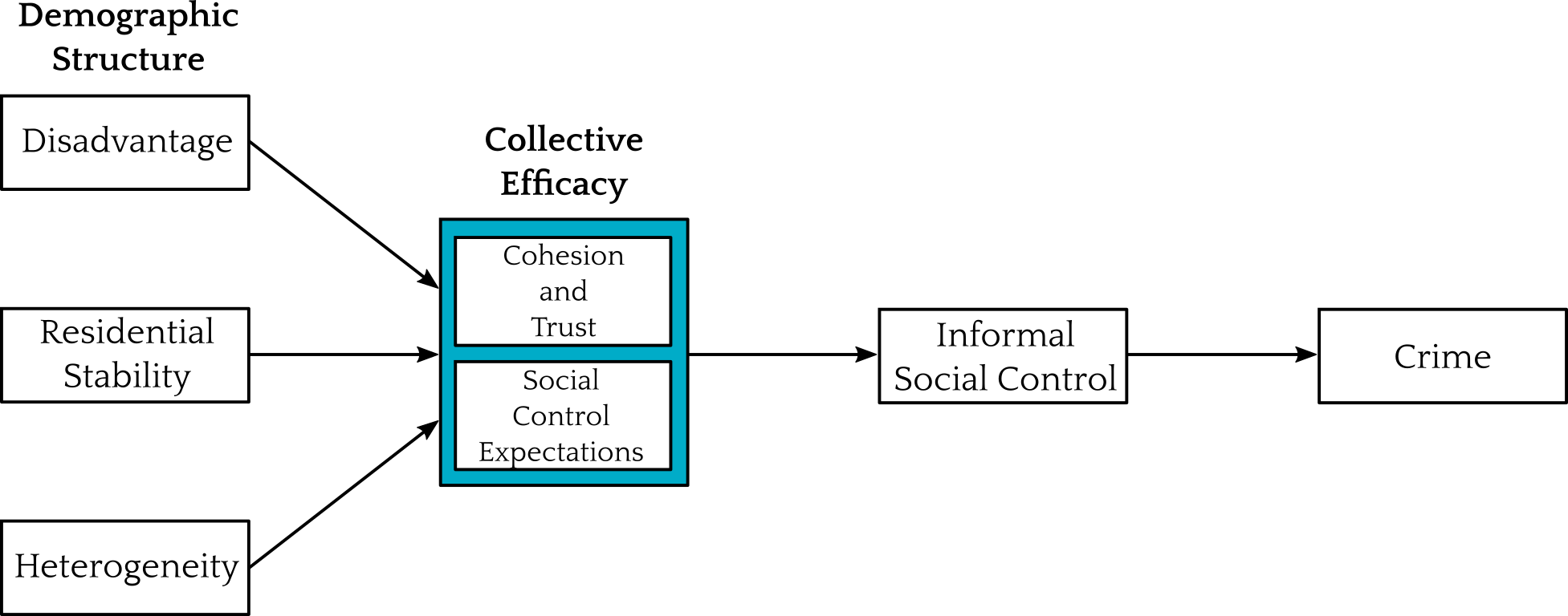 <br> .text-center[ *An explanation for crime differences between neighborhoods* ] --- ## Routine Activity The built environment explains why crime is concentrated in particular places within neighbourhoods: it influences opportunity <br>  <br> .text-center[ *An explanation for crime differences between locations* ] --- # From the paper My argument: Neighbourhoods with high collective efficacy in the past will have low crime in the present because they prevented and removed criminogenic features of the built environment <br> 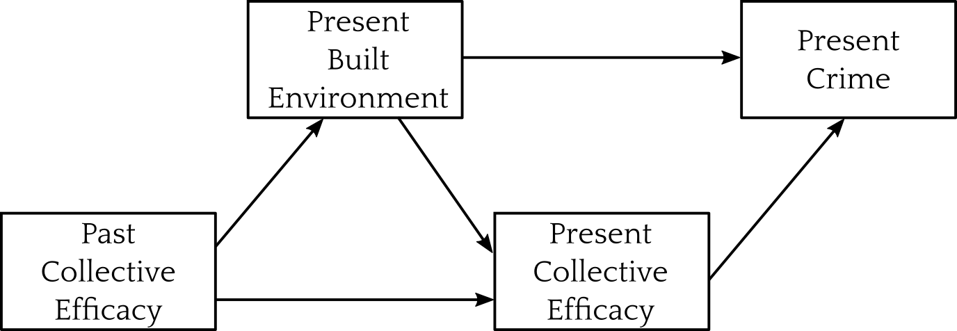 <br> .text-center[ *A link between neighborhood structures and place characteristics* ] --- # Chicago Data .pull-left[ Merged many datasets to test: * PHDCN Community Survey * 1995 Collective Efficacy * Chicago Community Adult Health Study (CCAHS) * 2001-2003 Collective Efficacy * 8 built environment features * Chicago Police Department reported crimes * Homicide / Gun Violence * Robbery * All violent crime * All property crime * City of Chicago street network * Longitudinal Tract DataBase * Demographic composition ] .pull-right[ 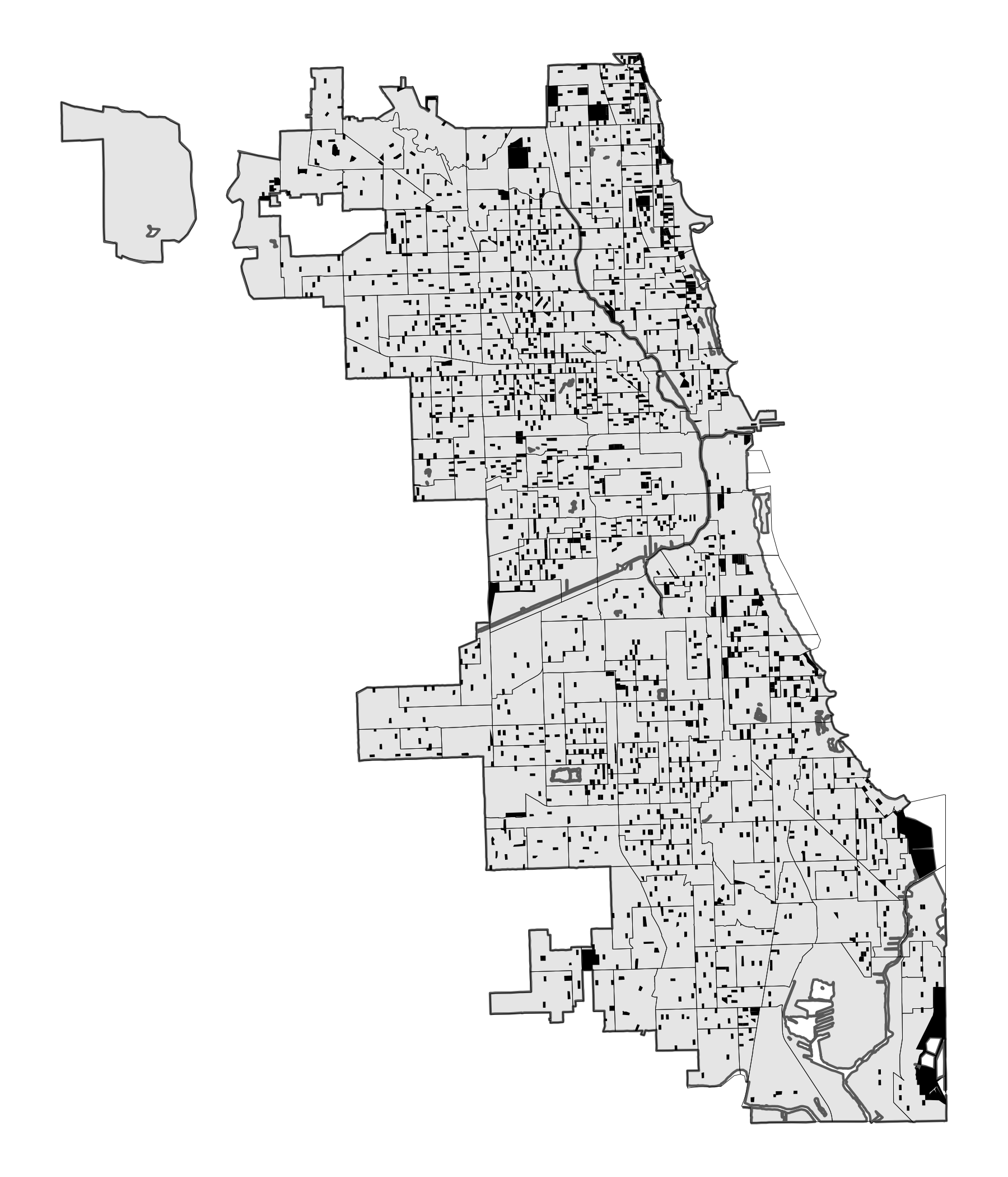 .center[*1641 blocks nested in 343 neighbourhood clusters*] ] --- # Loading Data ```r library(tidyverse) library(broom) *load(url("https://github.com/clanfear/built_environment_ce/raw/main/data/analytical_data/ccahs_block_analytical_unstd.RData")) ``` These are public replication data for [Lanfear, Charles C. (2022). Collective Efficacy and the Built Environment. *Criminology*, 60(2)](https://github.com/clanfear/built_environment_ce) These data describe: * 1641 city blocks in 343 Chicago neighborhoods * Crime in 2004–2006 * Survey data on collective efficacy in 1995 and 2001–2003 * Built environment from 2001–2003 * Proportions (0 to 1) of surrounding block faces * Census data from 2000 .footnote[ [1] `url()` tells `load()` to look online for the file; `read_csv()` does this automatically! ] --- .text-72[ ```r glimpse(ccahs_block_analytical_unstd) ``` ``` ## Rows: 1,641 ## Columns: 27 ## $ CRIME_homicide_2004_2006 <dbl> 0, 0, 0, 0, 1… ## $ CRIME_assault_battery_gun_2004_2006 <dbl> 1, 1, 6, 1, 1… ## $ CRIME_homicide_assault_battery_gun_2004_2006 <dbl> 1, 1, 6, 1, 2… ## $ CRIME_robbery_2004_2006 <dbl> 5, 1, 24, 6, … ## $ CRIME_violent_2004_2006 <dbl> 6, 3, 45, 8, … ## $ CRIME_property_2004_2006 <dbl> 30, 9, 138, 2… ## $ CE_hlm_1995 <dbl> -1.9127906, -… ## $ CE_hlm_2001 <dbl> -0.5537845, -… ## $ FAC_disadv_2000 <dbl> 0.2324679, 0.… ## $ FAC_stability_2000 <dbl> 0.7335206, 0.… ## $ FAC_hispimm_2000 <dbl> -0.2542902, -… ## $ density_ltdb_nc_2000 <dbl> 13863.7720, 1… ## $ BE_pr_commercial_block_2001 <dbl> 0.1666667, 0.… ## $ BE_pr_bar_onstreet_block_2001 <dbl> 0, 0, 0, 0, 0… ## $ BE_pr_liquor_onstreet_block_2001 <dbl> 0.00, 0.00, 0… ## $ BE_pr_vacant_onstreet_block_2001 <dbl> 0.0000000, 0.… ## $ BE_pr_abandoned_bld_onstreet_block_2001 <dbl> 0.00, 0.00, 0… ## $ BE_pr_commer_dest_onstreet_block_2001 <dbl> 0.0000000, 0.… ## $ BE_pr_recreation_block_2001 <dbl> 0.5000000, 0.… ## $ BE_pr_parking_block_2001 <dbl> 0.1666667, 0.… ## $ MIXED_LAND_USE_2001 <dbl> 0.00, 0.25, 0… ## $ orig_density_block <dbl> 13512.130, 10… ## $ street_class_near <dbl> 2, 1, 2, 1, 2… ## $ ccahs_nc <fct> 1, 1, 1, 1, 1… ## $ FAC_disadv_2000_2 <dbl> 0.05404133, 0… ## $ density_block <dbl> 8.651113e-03,… ## $ density_block_2 <dbl> -0.0151302783… ``` ] --- .text-72[ ```r ccahs_block_analytical_unstd |> select(where(is.numeric)) |> pivot_longer(everything()) |> group_by(name) |> summarize(across(value, list(mean = mean, sd = sd, min = min, max = max), .names = "{.fn}")) |> mutate(across(-name, ~round(.,2))) |> print(n=26) ``` ``` ## # A tibble: 26 × 5 ## name mean sd min max ## <chr> <dbl> <dbl> <dbl> <dbl> ## 1 BE_pr_abandoned_bld_onstreet_block_2001 0.12 0.21 0 1 ## 2 BE_pr_bar_onstreet_block_2001 0.05 0.13 0 1 ## 3 BE_pr_commer_dest_onstreet_block_2001 0.21 0.26 0 1 ## 4 BE_pr_commercial_block_2001 0.26 0.27 0 1 ## 5 BE_pr_liquor_onstreet_block_2001 0.03 0.1 0 0.75 ## 6 BE_pr_parking_block_2001 0.11 0.16 0 1 ## 7 BE_pr_recreation_block_2001 0.05 0.09 0 1 ## 8 BE_pr_vacant_onstreet_block_2001 0.12 0.21 0 1 ## 9 CE_hlm_1995 0 1 -2.93 3 ## 10 CE_hlm_2001 -0.02 1.01 -3.64 2.81 ## 11 CRIME_assault_battery_gun_2004_2006 1.02 1.75 0 18 ## 12 CRIME_homicide_2004_2006 0.1 0.35 0 4 ## 13 CRIME_homicide_assault_battery_gun_2004_2006 1.11 1.88 0 21 ## 14 CRIME_property_2004_2006 20.3 24.6 0 315 ## 15 CRIME_robbery_2004_2006 3.18 4.39 0 44 ## 16 CRIME_violent_2004_2006 6.42 8.34 0 79 ## 17 FAC_disadv_2000 0 0.47 -1.12 1.68 ## 18 FAC_disadv_2000_2 0.22 0.3 0 2.82 ## 19 FAC_hispimm_2000 0.03 0.51 -0.81 1.19 ## 20 FAC_stability_2000 0 0.48 -1.16 0.98 ## 21 MIXED_LAND_USE_2001 0.32 0.32 0 1 ## 22 density_block 0 0.02 -0.04 0.24 ## 23 density_block_2 0 0.02 -0.02 0.55 ## 24 density_ltdb_nc_2000 7196. 4419. 178. 31661. ## 25 orig_density_block 10853. 7590. 0 83420. ## 26 street_class_near 1.83 0.83 1 3 ``` ] --- ## The real model The actual model (set of models, really) is more complicated: 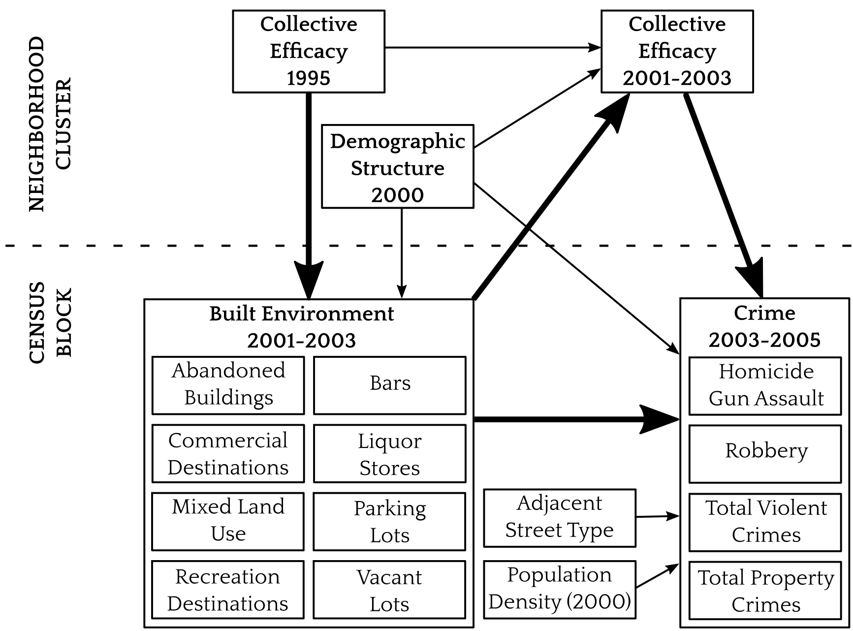 .text-center[ *We'll focus on total violent crimes* ] --- # Neighborhood Model ```r neighb_model <- lm(CRIME_violent_2004_2006 ~ CE_hlm_2001 + CE_hlm_1995 + FAC_disadv_2000 + FAC_stability_2000 + FAC_hispimm_2000, data = ccahs_block_analytical_unstd) ``` <!-- --> My theory says past collective efficacy predicts present crime... ...but only because of effects on the (unobserved) built environment --- ## Neighborhood Model Results .text-80[ ```r summary(neighb_model) ``` ``` ## ## Call: ## lm(formula = CRIME_violent_2004_2006 ~ CE_hlm_2001 + CE_hlm_1995 + ## FAC_disadv_2000 + FAC_stability_2000 + FAC_hispimm_2000, ## data = ccahs_block_analytical_unstd) ## ## Residuals: ## Min 1Q Median 3Q Max ## -17.397 -3.742 -1.280 1.779 69.743 ## ## Coefficients: ## Estimate Std. Error t value Pr(>|t|) ## (Intercept) 6.5186 0.1834 35.537 < 2e-16 *** ## CE_hlm_2001 -0.5159 0.2151 -2.398 0.0166 * ## CE_hlm_1995 -0.5639 0.2504 -2.252 0.0244 * ## FAC_disadv_2000 3.6753 0.4656 7.894 5.34e-15 *** ## FAC_stability_2000 3.6532 0.4699 7.775 1.33e-14 *** ## FAC_hispimm_2000 -3.2297 0.3765 -8.579 < 2e-16 *** ## --- ## Signif. codes: 0 '***' 0.001 '**' 0.01 '*' 0.05 '.' 0.1 ' ' 1 ## ## Residual standard error: 7.413 on 1635 degrees of freedom ## Multiple R-squared: 0.2116, Adjusted R-squared: 0.2092 ## F-statistic: 87.77 on 5 and 1635 DF, p-value: < 2.2e-16 ``` ] --- ## Neighborhood Model Results ```r neighb_model |> tidy() ``` ``` ## # A tibble: 6 × 5 ## term estimate std.error statistic p.value ## <chr> <dbl> <dbl> <dbl> <dbl> ## 1 (Intercept) 6.52 0.183 35.5 1.88e-205 ## 2 CE_hlm_2001 -0.516 0.215 -2.40 1.66e- 2 ## 3 CE_hlm_1995 -0.564 0.250 -2.25 2.44e- 2 ## 4 FAC_disadv_2000 3.68 0.466 7.89 5.34e- 15 ## 5 FAC_stability_2000 3.65 0.470 7.77 1.33e- 14 ## 6 FAC_hispimm_2000 -3.23 0.376 -8.58 2.19e- 17 ``` >If a block had been in a neighborhood with 1 unit higher collective efficacy in 2001, we'd expect to have seen about -0.516 fewer crimes there in 2004–2006, holding constant 1995 collective efficacy and year 2000 demographic composition. Note 1995 collective efficacy looks at least as strong as 2001 --- # Full Model The full model adds the built environment (opportunity) path: .text-80[ ```r full_model <- lm(CRIME_violent_2004_2006 ~ CE_hlm_2001 + CE_hlm_1995 + FAC_disadv_2000 + FAC_stability_2000 + FAC_hispimm_2000 + density_ltdb_nc_2000 + BE_pr_vacant_onstreet_block_2001 + BE_pr_abandoned_bld_onstreet_block_2001 + BE_pr_commer_dest_onstreet_block_2001 + BE_pr_recreation_block_2001 + BE_pr_parking_block_2001 + BE_pr_commercial_block_2001 + BE_pr_bar_onstreet_block_2001 + BE_pr_liquor_onstreet_block_2001 + density_block + I(density_block^2) + street_class_near, data = ccahs_block_analytical_unstd) ``` ] <!-- --> .footnote[ Note that only arrows going into **Crime** go into the model formula ] --- ## Full Model Results There are many parameters, so `tidy()` it up: .text-80[ ```r tidy(full_model) |> mutate(across(-term, ~round(., 3))) ``` ``` ## # A tibble: 18 × 5 ## term estimate std.error statistic p.value ## <chr> <dbl> <dbl> <dbl> <dbl> ## 1 (Intercept) 1.13 0.605 1.87 0.062 ## 2 CE_hlm_2001 -0.311 0.205 -1.52 0.129 ## 3 CE_hlm_1995 -0.096 0.249 -0.384 0.701 ## 4 FAC_disadv_2000 4.63 0.502 9.21 0 ## 5 FAC_stability_2000 0.872 0.508 1.72 0.086 ## 6 FAC_hispimm_2000 -3.88 0.4 -9.68 0 ## 7 density_ltdb_nc_2000 0 0 2.40 0.016 ## 8 BE_pr_vacant_onstreet_block… -0.5 0.882 -0.566 0.571 ## 9 BE_pr_abandoned_bld_onstree… 3.12 0.962 3.25 0.001 ## 10 BE_pr_commer_dest_onstreet_… 3.84 1.15 3.36 0.001 ## 11 BE_pr_recreation_block_2001 6.48 1.93 3.35 0.001 ## 12 BE_pr_parking_block_2001 1.99 1.19 1.68 0.093 ## 13 BE_pr_commercial_block_2001 0.497 1.09 0.455 0.649 ## 14 BE_pr_bar_onstreet_block_20… -1.44 1.53 -0.944 0.345 ## 15 BE_pr_liquor_onstreet_block… 3.14 1.98 1.59 0.113 ## 16 density_block 69.9 12.6 5.54 0 ## 17 I(density_block^2) -382. 106. -3.61 0 ## 18 street_class_near 1.57 0.24 6.54 0 ``` ] --- # Comparing models .text-80[ ```r anova(neighb_model, full_model) |> tidy() ``` ``` ## # A tibble: 2 × 7 ## term df.residual rss df sumsq statistic p.value ## <chr> <dbl> <dbl> <dbl> <dbl> <dbl> <dbl> ## 1 CRIME_violent… 1635 89849. NA NA NA NA ## 2 CRIME_violent… 1623 79069. 12 10780. 18.4 7.03e-38 ``` ] The model fits quite a bit better; `\(R^2\)` increases from 0.21 to 0.31 too -- .text-80[ ```r tidy(full_model) |> mutate(across(-term, ~round(., 3))) |> filter(str_detect(term, "CE")) ``` ``` ## # A tibble: 2 × 5 ## term estimate std.error statistic p.value ## <chr> <dbl> <dbl> <dbl> <dbl> ## 1 CE_hlm_2001 -0.311 0.205 -1.52 0.129 ## 2 CE_hlm_1995 -0.096 0.249 -0.384 0.701 ``` ] * 2001 collective efficacy dropped from -0.516 to -0.311 (-40%) * 1995 collective efficacy dropped from -0.564 to -0.096 (-83%) .text-center[ *Built environment features mostly wipe out 1995 CE!* ] --- # Non-Linearity Note that there was a **quadratic** term on block-level population density. Why did I include that? -- 1. There are some theoretical reasons to expect it 2. It fixed some non-linearity in the residuals 3. It fit quite a bit better: .text-80[ ```r full_noquad_model <- lm(CRIME_violent_2004_2006 ~ CE_hlm_2001 + CE_hlm_1995 + FAC_disadv_2000 + FAC_stability_2000 + FAC_hispimm_2000 + density_ltdb_nc_2000 + density_block + street_class_near + BE_pr_vacant_onstreet_block_2001 + BE_pr_abandoned_bld_onstreet_block_2001 + BE_pr_commer_dest_onstreet_block_2001 + BE_pr_recreation_block_2001 + BE_pr_parking_block_2001 + BE_pr_commercial_block_2001 + BE_pr_bar_onstreet_block_2001 + BE_pr_liquor_onstreet_block_2001, data = ccahs_block_analytical_unstd) anova(full_noquad_model, full_model) |> tidy() |> mutate(p.value = round(p.value, 3)) ``` ``` ## # A tibble: 2 × 7 ## term df.residual rss df sumsq statistic p.value ## <chr> <dbl> <dbl> <dbl> <dbl> <dbl> <dbl> ## 1 CRIME_violent_20… 1624 79705. NA NA NA NA ## 2 CRIME_violent_20… 1623 79069. 1 636. 13.0 0 ``` ] --- ## Quadratic Interpretation ```r full_model |> tidy() |> filter(str_detect(term, "density_block")) |> mutate(p.value = round(p.value, 3)) ``` ``` ## # A tibble: 2 × 5 ## term estimate std.error statistic p.value ## <chr> <dbl> <dbl> <dbl> <dbl> ## 1 density_block 69.9 12.6 5.54 0 ## 2 I(density_block^2) -382. 106. -3.61 0 ``` Effect of density: 69.87 -763*`density_block` -- ```r ccahs_block_analytical_unstd |> pull(density_block) |> round(3) %>% {setNames(c(min(.), median(.), max(.)), c("min", "mean", "max"))} ``` ``` ## min mean max ## -0.035 -0.006 0.236 ``` Effect of density at its max: `\(69.87 -763*0.236\)` = `\(-110.198\)` --- # Moderation or Interaction We introduce **interaction terms** when we want to know if effects differ by... * Groups * Contexts (e.g., neighborhood) * Characteristics (e.g., capability) -- A reviewer asked if disadvantage (a context) **moderated** block-level built environment effects—a common finding in the opportunity literature * e.g., do some features only produce crime in highly disadvantaged neighborhoods? I tested this—and we can too! --- ## Moderation test .text-80[ ```r full_int_model <- lm(CRIME_violent_2004_2006 ~ CE_hlm_2001 + CE_hlm_1995 + FAC_disadv_2000 + FAC_stability_2000 + FAC_hispimm_2000 + density_ltdb_nc_2000 + density_block + density_block_2 + street_class_near + FAC_disadv_2000*BE_pr_vacant_onstreet_block_2001 + FAC_disadv_2000*BE_pr_abandoned_bld_onstreet_block_2001 + FAC_disadv_2000*BE_pr_commer_dest_onstreet_block_2001 + FAC_disadv_2000*BE_pr_recreation_block_2001 + FAC_disadv_2000*BE_pr_parking_block_2001 + FAC_disadv_2000*BE_pr_commercial_block_2001 + FAC_disadv_2000*BE_pr_bar_onstreet_block_2001 + FAC_disadv_2000*BE_pr_liquor_onstreet_block_2001, data = ccahs_block_analytical_unstd) anova(full_int_model, full_model) |> tidy() ``` ``` ## # A tibble: 2 × 7 ## term df.residual rss df sumsq statistic p.value ## <chr> <dbl> <dbl> <dbl> <dbl> <dbl> <dbl> ## 1 CRIME_violent_20… 1615 78354. NA NA NA NA ## 2 CRIME_violent_20… 1623 79069. -8 -716. 1.84 0.0651 ``` ] Some evidence for moderation, but not strong enough to warrant inclusion! I did toss the results in the appendix though --- ## oh no .text-60[ ```r full_int_model |> tidy() |> print(n=26) ``` ``` ## # A tibble: 26 × 5 ## term estimate std.error statistic p.value ## <chr> <dbl> <dbl> <dbl> <dbl> ## 1 (Intercept) 8.42e-1 0.601 1.40 1.61e- 1 ## 2 CE_hlm_2001 -3.43e-1 0.207 -1.66 9.74e- 2 ## 3 CE_hlm_1995 -1.43e-1 0.250 -0.572 5.68e- 1 ## 4 FAC_disadv_2000 3.80e+0 0.760 5.00 6.48e- 7 ## 5 FAC_stability_2000 6.86e-1 0.520 1.32 1.88e- 1 ## 6 FAC_hispimm_2000 -3.80e+0 0.414 -9.17 1.41e-19 ## 7 density_ltdb_nc_2000 1.38e-4 0.0000550 2.51 1.21e- 2 ## 8 density_block 4.57e+1 9.11 5.01 5.95e- 7 ## 9 density_block_2 -2.99e+1 7.70 -3.89 1.05e- 4 ## 10 street_class_near 1.56e+0 0.241 6.49 1.17e-10 ## 11 BE_pr_vacant_onstreet_bloc… -6.04e-1 0.906 -0.666 5.05e- 1 ## 12 BE_pr_abandoned_bld_onstre… 2.88e+0 1.21 2.37 1.78e- 2 ## 13 BE_pr_commer_dest_onstreet… 3.75e+0 1.15 3.27 1.10e- 3 ## 14 BE_pr_recreation_block_2001 6.70e+0 1.93 3.47 5.41e- 4 ## 15 BE_pr_parking_block_2001 2.00e+0 1.19 1.68 9.36e- 2 ## 16 BE_pr_commercial_block_2001 6.34e-1 1.10 0.578 5.63e- 1 ## 17 BE_pr_bar_onstreet_block_2… -2.74e+0 1.66 -1.64 1.01e- 1 ## 18 BE_pr_liquor_onstreet_bloc… 2.91e+0 1.99 1.46 1.43e- 1 ## 19 FAC_disadv_2000:BE_pr_vaca… 6.92e-1 1.84 0.377 7.06e- 1 ## 20 FAC_disadv_2000:BE_pr_aban… 6.44e-1 2.35 0.275 7.84e- 1 ## 21 FAC_disadv_2000:BE_pr_comm… 2.03e+0 2.28 0.890 3.74e- 1 ## 22 FAC_disadv_2000:BE_pr_recr… 4.83e+0 3.52 1.37 1.69e- 1 ## 23 FAC_disadv_2000:BE_pr_park… 3.45e-1 2.22 0.156 8.76e- 1 ## 24 FAC_disadv_2000:BE_pr_comm… 1.15e-1 2.16 0.0531 9.58e- 1 ## 25 FAC_disadv_2000:BE_pr_bar_… -9.31e+0 3.43 -2.72 6.65e- 3 ## 26 FAC_disadv_2000:BE_pr_liqu… 8.03e+0 3.87 2.08 3.81e- 2 ``` ] --- ## Moderation complications What is the effect of abandoned buildings? ```r full_int_model |> tidy() |> filter(str_detect(term, "abandoned")) ``` ``` ## # A tibble: 2 × 5 ## term estimate std.error statistic p.value ## <chr> <dbl> <dbl> <dbl> <dbl> ## 1 BE_pr_abandoned_bld_onstreet… 2.88 1.21 2.37 0.0178 ## 2 FAC_disadv_2000:BE_pr_abando… 0.644 2.35 0.275 0.784 ``` `\(2.88 + 0.64*Disadvantage\)` * 2.24 when `\(Disadvantage\)` is -1 * 2.88 when `\(Disadvantage\)` is 0 * 3.52 when `\(Disadvantage\)` is 1 -- But wait, what's the effect of Disadvantage? --- ## oh noooo Unfortunately, it depends on *every built environment feature*! .pull-left[ .text-80[ ```r full_int_model |> tidy() |> filter(str_detect(term, "disadv")) |> select(term, estimate) |> print(width=40) ``` ``` ## # A tibble: 9 × 2 ## term estimate ## <chr> <dbl> ## 1 FAC_disadv_2000 3.80 ## 2 FAC_disadv_2000:BE_pr_vacant… 0.692 ## 3 FAC_disadv_2000:BE_pr_abando… 0.644 ## 4 FAC_disadv_2000:BE_pr_commer… 2.03 ## 5 FAC_disadv_2000:BE_pr_recrea… 4.83 ## 6 FAC_disadv_2000:BE_pr_parkin… 0.345 ## 7 FAC_disadv_2000:BE_pr_commer… 0.115 ## 8 FAC_disadv_2000:BE_pr_bar_on… -9.31 ## 9 FAC_disadv_2000:BE_pr_liquor… 8.03 ``` ] ] .pull-right[ Partial derivative with respect to disadvantage: `\(\;3.798217\)`<br> `\(+ (0.692238 * vacant)\)`<br> `\(+ (0.6444968 * abandoned)\)`<br> `\(+ (2.0297129 * commer)\)`<br> `\(+ (4.8349173 * recreation)\)`<br> `\(+ (0.3453893 * parking)\)`<br> `\(+ (0.1145244 * commercial)\)`<br> `\(+ (-9.3090589 * bar)\)`<br> `\(+ (8.0312971 * liquor)\)`<br> ] .text-center[ *This would be bad if we were mainly interested in disadvantage!* ] --- class: inverse # More Advanced Things > Any sufficiently advanced technology is indistinguishable from magic – Sir Arthur C. Clarke --- ## Alternate approaches .pull-left[ .text-85[ ```r full_model |> augment() |> ggplot(aes(x = .fitted, y = .resid)) + geom_point() + geom_smooth() ``` <!-- --> ] ] .pull-right[ It doesn't look like our model is doing great Multiple issues: * No negative values; a count variable! * Zeroes: Can't log! * Non-linearity * Heteroskedasticity ] -- These suggest a *better* model; something in the **Poisson** family¹ You can learn about these in SSRMP modules or textbooks .footnote[ [1] I used a hierarchical negative binomial model in this paper ] --- ## Common ones to consider * **Poisson** regression (and related approaches) * Counts and other non-negative outcomes * Multiplicative relationships * Interested in rates -- * **Binomial**, e.g., logit / logistic regression * Binary (0/1) or fractional outcomes (0–1) * Interested in probabilities -- * **Event history** or hazard models * Duration outcomes, e.g., time to death * Censored data, e.g., with some alive at last follow-up * Transitions between states, e.g., incarcerated to free (and back) -- * **Hierarchical models** * Nested data, e.g., blocks in neighborhoods * Repeated observations, e.g., person-years * **Time series** and **panel models** are included here --- ## Mediation  <br> We test for **mediation** when we want to know if an effect works through a *particular* front door, e.g., `\(X \rightarrow Z \rightarrow Y\)` -- Mediation requires strong assumptions (sequential ignorability): * You've identified the effect of `\(X \rightarrow Z\)` * You've also identified `\(Z \rightarrow Y\)` This is *very hard* to do, but if you want to do it, read VanderWeele (2015) *Explanation in Causal Inference: Methods for Mediation and Interaction* --- ## Fixed Effects One problem with my analysis is I don't observe *change* in the built environment—I only had one time point! * There might be unmeasured differences between neighborhoods or blocks explaining my effects * If I'd had at least two measures, I could make a more convincing test by *looking only at changes* -- **Fixed effects** or **unobserved effects** models are one way to do this: * Introduce a categorical variable with a level for *every unit* and/or time period * e.g., 31 borough dummies in our `metro_2021` data * This "controls" for *mean differences* between the units * i.e., it adjust for anything *stable over time* * This is a type of **hierarchical model** * Specifically, one where fixed characteristics of units are a *nuisance* -- This is *very easy* and *very common*, but see Huntington-Klein chapter 16 for more --- # Book Recommendations * R Programming * Grolemund & Wickham (2024) *R for Data Science* * Bryan et al. (2023) *What They Forgot to Teach You About R* * Healy (2018) *Data Visualization: A Practical Introduction* * Basic Stats with Programming * Çetinkaya-Rundel & Hardin (2023) *Introduction to Modern Statistics* * Llaudet & Imai (2022) *Data Analysis for Social Science* * Causal Inference * Morgan & Winship (2014) *Counterfactuals and Causal Inference* * Cunningham (2021) *Causal Inference: The Mixtape* --- class: inverse # Wrap-Up * Assignment 2 due Sunday 11:59 ## Freedom