class: center, top, title-slide .title[ # Causality and Theory Testing ] .subtitle[ ## CRM Week 4 ] .author[ ### Charles Lanfear ] .date[ ### 4 Nov 2025<br>Updated: 02 Nov 2025 ] --- # Today * What is causality anyway? * Causal graphs * Types of paths * An example * Theory testing * Turning theories into graphs * Turning graphs into estimators --- class: inverse # Causality  --- # Perspectives .pull-left-60[ Different philosophical perspectives * Probabilistic * Manipulation * Mechanistic * **Counterfactual** For a primer, consider Illari & Russo ] .pull-right-40[  ] --- # Counterfactual Causality `\(X\)` causes `\(Y\)` if changing *only* `\(X\)` would change `\(Y\)` -- ‍This is quite broad: * `\(X\)` is typically not the only cause * e.g., `\(X\)` and `\(Z\)` can both be causes of `\(Y\)` -- * `\(X\)` may cause `\(Y\)` for multiple reasons * e.g., `\(X\)` may cause `\(Z\)` which causes `\(Y\)` ( `\(Z\)` is a *mechanism*) -- * `\(X\)` may only cause `\(Y\)` in certain contexts * e.e., `\(X\)` may cause `\(Y\)` only when `\(Z\)` is present -- .text-center[ *All that matters for the relationship to be causal is that if the distribution of `\(X\)` was different, it would result in a different distribution of `\(Y\)`* ] -- We call the process of estimating a causal effect **identification** --- # Theory and Causes Scientific theories are causal<sup>1</sup>: *They explain **why** things happen* .footnote[[1] This is subject to some debate] -- In criminology: * "Increasing the perceived risk of being caught reduces the likelihood of a person committing a particular crime" * "Increasing a person's self-control reduces their involvement in all crime" * "Learning violent definitions of situations increases a person's likelihood of using violence" * "Strong social institutions in neighbourhoods reduce crime" -- These are all testable, causal propositions about how the world works -- Theory testing is **causal inference**: Drawing *causal conclusions* from data * Doing this convincingly requires identifying causal effects --- # The Problem Let's say we want to know if we can reduce crime by clearing vacant lots * We want to identify the effect of lot clearing on crime -- But we only see *one outcome* per lot:<sup>1</sup> * If we clear a lot, we don't see what happens if we had not. * If we *don't* clear it, we don't see what happens if we had. .footnote[[1] This is often called the "fundamental problem of causal inference"] -- We call whichever outcome we don't see a **counterfactual**—it is counter to the fact of what actually happened -- Causal effects are *differences* between these **potential outcomes**: 1. What actually happened, which we see (factual) 2. An alternative, which we do not observe (counterfactual) --- # Potential Outcomes <br>  -- .text-center[ *How do we calculate a difference when we only see one outcome?* ] --- # Between Comparison .pull-left[ We could compare two lots: * **One cleared (T=1)** * .strong-blue[One not cleared (T=0)] And use the difference in crime (δT) as a causal effect ] .pull-right[  ] -- *What if the difference is because the lots are different?* -- * We could compare only lots that look *identical* -- *But if those lots are identical, why did one get cleared and not the other?* * We might have missed an important difference * We wouldn't be sure unless we knew *why* each lot got cleared --- # Put another way <br>  --- # Within Comparison .pull-left[ We could compare the same lot: * **After clearing (T=1)** * .strong-blue[Before clearing (T=0)] And use the before-and-after crime difference (δT) as a causal effect ] .pull-right[  ] -- *But what if the crime change was going to happen anyway?* * The clearing simply coincided with the crime change * Worse, maybe the change in crime *caused the clearing* -- *Or, what if the lot was cleared **because** it would make a difference here?* * What if there would be no difference for *other* lots? --- # Potential Outcomes .pull-left[ All of these problems are really one problem: *Differences in **potential outcomes** between cleared and uncleared lots* ] .pull-right[  ] -- These problems are resolved if the potential outcomes for cleared and uncleared lots are *the same on average* (unrelated to the treatment) -- The average difference in outcomes between treatment and control groups then provides an unbiased estimate of the causal effect (the estimand) -- .text-center[ *How do we make sure the cleared and uncleared lots are the same?* ] --- # Randomization *Randomized controlled trials do this* * Take a relatively large number of lots -- * Randomly assign treatment: clear some lots but not others -- * On average, cleared and uncleared lots will be similar *in every way except for clearing* -- Randomization makes treatment **independent** of potential outcomes * Clearing is equally likely no matter how much a lot would benefit -- If we randomly assign a treatment, we can estimate a causal effect as the average difference in outcomes between treated groups * We call this the **average treatment effect** (**ATE**) * You can calculate this with a *cross-tab* -- .text-center[ *What if we're interested in things we can't randomly assign?* ] --- # Back to the DGP When we can't **randomize**, we need to **theorize** -- We need to figure out the **data generating process** for our treatment and outcome * What makes some units get treated? * What makes treatment more (or less) effective for some units? -- This requires making **assumptions**, which are part of your **model**<sup>1</sup> * `\(Z\)` is unrelated to `\(X\)` * `\(B\)` only causes `\(Y\)` through `\(C\)` .footnote[[1] RCTs also make many assumptions, but they're usually weaker and fewer] -- .text-center[ *If our model is correct, it tells us exactly how to identify the causal effect* ] -- .text-center[ *So how do we make the model?* ] --- class: inverse # Directed Acyclic Graphs  --- # Causal Graphs .pull-left[ Classic statistics is mathy, using things like this: `$$Y = f(X,Z)$$` ... to say `\(Y\)` is caused by a combination of `\(X\)` and `\(Z\)` ] -- .pull-right[ We're going to work with **directed acyclic graphs** (DAGs) instead: <!-- --> ] -- Directed acyclic graphs have pretty simple rules: * Arrows between variables point from causes to outcomes (directed) -- * No arrow means no direct causal relationship -- * Something can't cause itself... *even through other things* (acyclic) -- .text-center[ *DAGs are a way to write out a model that tells you how to identify effects* ] --- # Paths .pull-left[ A **path** is any set of arrows linking two variables together There are three paths from `\(X\)` to `\(Y\)`: * `\(X \rightarrow Y\)` * `\(\color{#003C71}{X \leftarrow Z \rightarrow Y}\)` * `\(\color{#8A1538}{X \rightarrow W \leftarrow Y}\)` ] .pull-right[ <!-- --> ] -- Let's say we want to know the effect of `\(X\)` on `\(Y\)` * Paths where all arrows point from `\(X\)` to `\(Y\)` are called **front doors** * Paths where arrows point to both `\(X\)` to `\(Y\)` are **back doors** * Paths where arrows point *at* each other are **colliders** -- .text-center[ We estimate effects *through front doors* by closing *all back doors* and *avoiding collisions* ] --- # Closing Back Doors Variables that open back doors are called **confounders** * Confounders cause *dependence between treatment and potential outcomes* -- We close doors by **adjusting**, **controlling**, or **holding constant** variables along the path—either by design or in our statistical estimator<sup>1</sup> .footnote[[1] We'll see this in a bit] -- .pull-left[ Adjusting for Z closes the back door The only remaining path is the front door we're interested in The effect of `\(X\)` on `\(Y\)` is identified ] .pull-right[ <!-- --> ] --- # More Front Doors Very often your model has multiple front doors -- You don't adjust for these—they're ways `\(X\)` impacts `\(Y\)`! * We call these **mechanisms** or **mediators** -- .pull-left[ There are *two* front doors * `\(X \rightarrow Y\)` * `\(X \rightarrow A \rightarrow Y\)` We've adjusted for `\(Z\)` but not `\(A\)` The effect of `\(X\)` on `\(Y\)` is identified! ] .pull-right[ <!-- --> ] -- The *total* estimated effect of `\(X\)` on `\(Y\)` will be the sum of all front door paths leading between them. --- # Colliders Colliders are the *opposite* of back door paths: They *block* associations from going down their path *unless we adjust for them* -- If you control for a collider on the path between `\(X\)` and `\(Y\)`, it opens the association back up and *introduces bias* -- .pull-left[ Adjusting for Z closes the back door But here we've adjusted for `\(W\)` too Now our estimate of `\(X \rightarrow Y\)` contains parts of `\(Y \rightarrow W\)` and `\(X \rightarrow W\)` ] .pull-right[ <!-- --> ] -- Controlling for a collider is sometimes **conditioning on a post-treatment variable** or **Berkson's paradox**, and is one form of **selection bias**. --- ## Collider Bias *Do people commit more crime when they're good at it?* <!-- --> <!-- --> --- # Unobservabed Variables A DAG *must* accurately represent what we think the data generating process is to be useful -- Sometimes we know a variable is important but we can't measure it -- .pull-left[ Unobserved variables are often indicated with circles Because they're unobserved, we can't adjust for them *directly* Here we can still block the path through `\(W\)` by adjusting for `\(Z\)` ] .pull-right[ <!-- --> ] -- Most of the time we can't observe *everything* that matters, but rigorous research will acknowledge this -- .text-center[ *This is all very abstract, so let's put them to work* ] --- class: inverse # DAGs at Work  --- # Measuring Bias in Policing 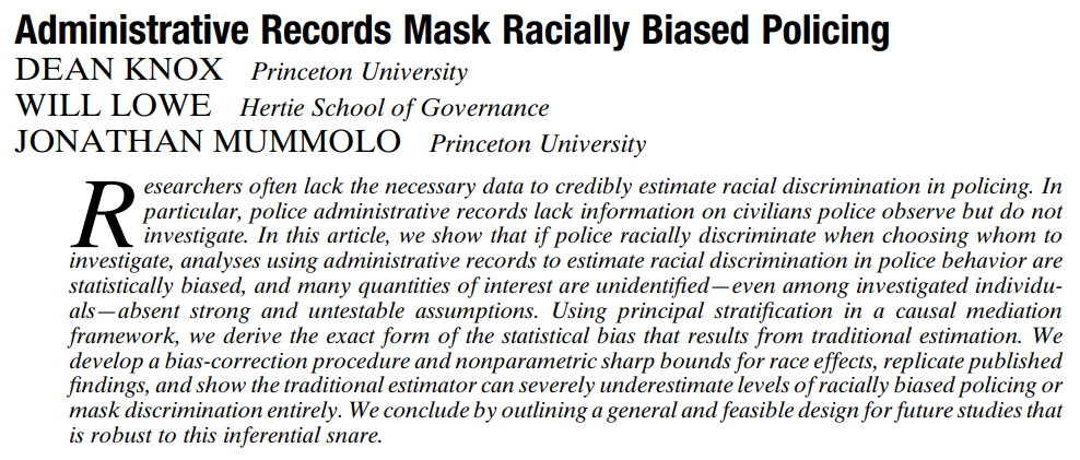 --- # Use of Force ‍Question: *Do US police use more force against black civilians?* -- Imagine you sample police encounters **identical** except for race *But* suppose bias leads police to: * Stop white civilians only for crimes * Stop black civilians with or without a crime -- Then, discard data on anyone police observed but *did not stop*. You are now comparing use of force between two groups: * White people committing crime * Black people committing no crime *or* committing a crime -- If use of force were the **same**, *we'd have a serious problem* -- *This is what police data actually show: we only see the stopped people!* --- # What We Want <!-- --> ‍Question: How does race impact officer decisions to use force? -- We could compare how often force is used on white vs. black subjects -- We could even get sophisticated: * Compare similar encounters * Compare similar subjects * Compare similar officers -- .text-center[ *Good ideas, but none of them will help* ] --- 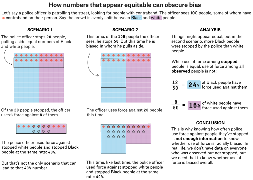 .footnote[ Source: [Bronner (2020) "Why statistics don’t capture the full extent of the systemic bias in policing"](https://fivethirtyeight.com/features/why-statistics-dont-capture-the-full-extent-of-the-systemic-bias-in-policing/) ] --- # The Problem <!-- --> ‍Problem: Race impacts likelihood of being stopped in the first place, but *we never see unstopped people* * We've conditioned on *being stopped*—a mediator! * We've blocked part of our front door! -- We can't identify the causal effect! --- # It Gets Worse <!-- --> More problems * Racial composition varies by neighborhood * Police deployments and strategy vary by neighborhood * Reasonable suspicion predicts both stops and use of force—and can't be observed --- # Consequences * Detecting bias in the decision to stop is difficult -- * If any stop bias exists, it is difficult to measure bias in...<sup>1</sup> * Arrests * Use of force * Frisks * Shootings .footnote[[1] Clever use of plausible assumptions can allow *bounded identification* that indicates substantial use of force bias by US police] -- * Raw numbers can easily show *opposite patterns* from underlying reality * Studies showing no bias—or anti-white bias—get *lots* of media, social media, and political traction --- class: inverse # Theory Testing  .footnote[Source: Adapted from Bursik & Grasmick 1993] --- # Recursive Models Criminological theories tell us how to construct DAGs -- Often this is fairly explicit, such as when authors provide a causal diagram... *and it already obeys DAG rules* -- 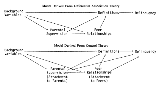 .footnote[Source: [Matsueda (1982)](https://doi.org/10.2307/2095194)] --- # Nonrecursive Models This is less clear when the causal diagram provided doesn't conform to DAG rules -- 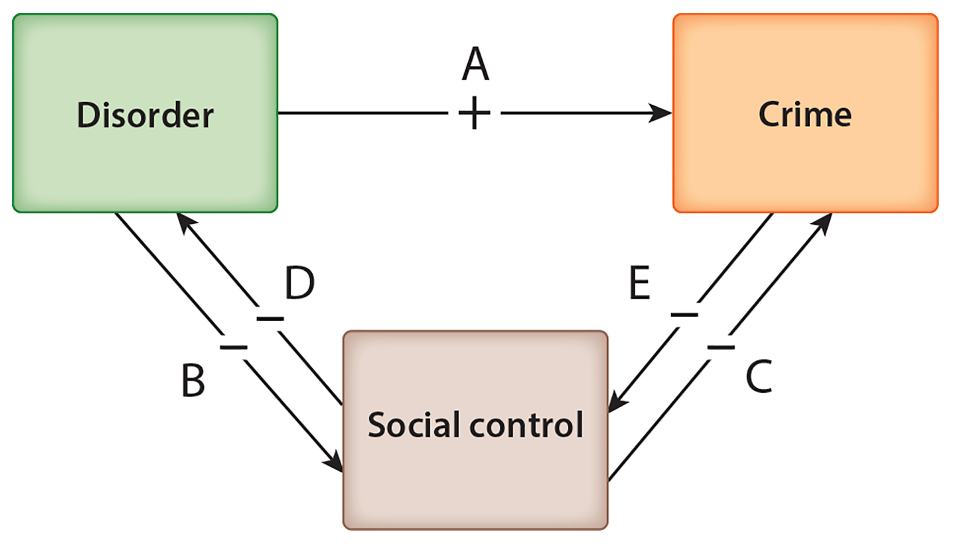 .footnote[Source: [Lanfear, Matsueda, & Beach (2018)](https://doi.org/10.1146/annurev-criminol-011419-041541)] -- Converting a model with **cycles** into an **acyclic** one can take some thought -- .text-center[ *All causal relationships really are acyclic though* ] --- # Broken Windows DAG Usually the trick to converting a cyclic graph to an acyclic one is realizing effects *occur over **time*** * This requires assumptions about (relative) timing <!-- --> -- Another way is through **intervening** or **cross-level** mechanisms * Many macro theories are circular without individual-level mechanisms --- # No Graphical Model Making a DAG is least clear when the authors provide no graphical representation of the model at all<sup>1</sup> .footnote[[1] Or when you're developing something new yourself!] -- * Record all the core variables they use * e.g., self control -- * Make note of causal statements * e.g., "self control **influences** crime by..." * Make these into arrows! -- * Try to reconcile circular paths * Consider temporal order * Consider cross-level mechanisms --- class: inverse # From DAG to Estimator  --- # Estimating Causal Effects Once you have a DAG, it is remarkably easy to proceed to an estimator -- Figure out what you can and cannot measure -- .pull-left[ If your measures let you close all back doors... * Adjust for back doors * Don't adjust for colliders or mechanisms * Choose appropriate method * Estimate the causal effect ] -- .pull-right[ If you can't close all back doors, either... * Close what you can and estimate an association * Might be *close* to identified! * *Give up* * **Get clever** ] -- ‍Remember: *clever estimation techniques are a last resort for problems with research design* It is *always* better to solve hard problems with *design* --- class: inverse # Controlling for Variables  --- # Regression Again So far we've just fit a simple straight line using one variable predicting another .pull-left[ |Term | Estimate| |:-----------|--------:| |Pop Density | 3.09| |(Intercept) | -20.78| ] .pull-right[ <!-- --> ] This doesn't get us very far for testing theories -- But there's no reason to have only one predictor --- # Multiple Predictors When we add predictors, we are **adjusting** or **controlling** for them to identify the effect we're interested in .pull-left[ |Term | Estimate| |:-----------|--------:| |Urban | -3.39| |Pop Density | 3.36| |(Intercept) | -23.04| ] .pull-right[ <!-- --> ] New interpretations: * "The association between density and crime, adjusting for area type" * "The average crime rate difference between urban and rural areas, adjusting for population density" -- .text-center[ *We could argue this is causal if we think the diagram is complete* ] --- # How it Works 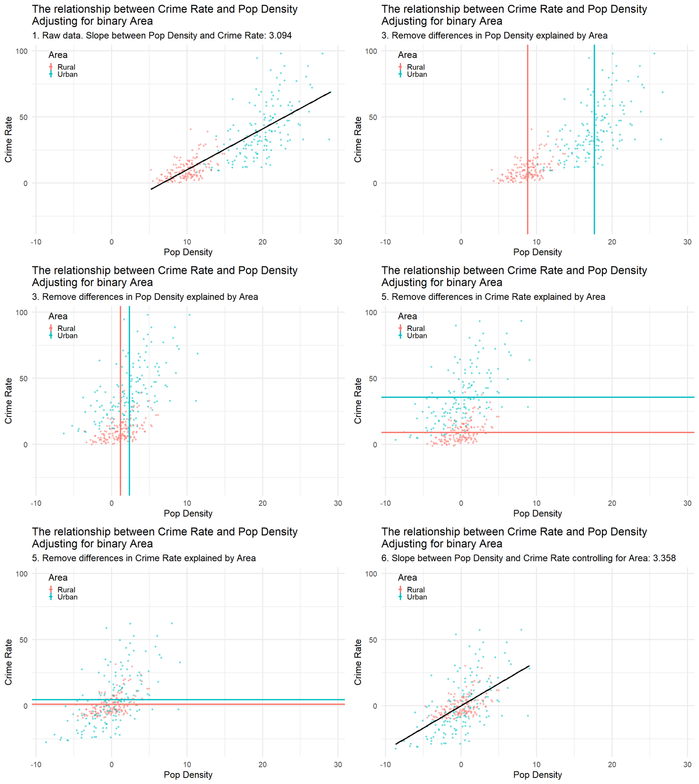 .footnote[Adapted from [`NickCH-K/causalgraphs`](https://github.com/NickCH-K/causalgraphs/blob/master/Animation%20of%20Controlling%20for%20Z.R)] --- # More Variables The same basic principle applies when more variables are introduced A verbal interpretation can sometimes get difficult .pull-left[ |Term | Estimate| |:---------------|--------:| |Urban | -2.19| |Pop Density | 3.11| |Incarc.: Medium | -6.45| |Incarc.: Low | -5.42| |(Intercept) | -15.97| ] -- .pull-right[ <!-- --> ] But a graph always fully encodes our expectations about relationships<sup>1</sup> .footnote[[1] If we're not sure how two variables are related, sometimes we just assume there is an unobserved (U) confounder connecting them] -- .text-center[ *What paths are actually identified if this model is true?* ] --- # Interpreting Controls DAGs highlight one of the most common mistakes made in empirical research: *Researchers often write as if every path is identified* * Interpreting the main "effect" as adjusted for covariates * Interpreting all covariates as adjusted for everything else -- .text-center[ *In general, these interpretations are logically impossible* *Usually, at most **one path** is identified* ] -- The purpose of **controls** is to close back doors, not to add additional interpretable causal paths * If a variable closes a back door, by definition its effect on the outcome is not identified * Control variable associations are typically not worth interpreting<sup>1</sup> .footnote[ [1] Reviewers or editors may make authors do this. Savvy authors will describe them appropriately. ] --- # Other Assumptions DAGs do not make **parametric** assumptions about relationships, such as: * Straight lines (versus curves) * Additive effects (versus multiplicative) * Error distributions -- In contrast, all estimation techniques make some sort of assumptions about how relationships should be calculated So far our estimators have been straight lines with independent effects that add together -- Common modifications to these methods include: * Polynomials or splines (curved lines) * Interaction / multiplicative terms (group-specific slopes) * Different error distributions (e.g., Poisson) -- .text-center[ *These are important but beyond the level of this course* ] --- # Causal Qualitative Research DAGs aren't just non-parametric—they are not necessarily quantitative -- DAGs can be useful for thinking through qualitative research too -- In particular, propositional (hypothesis testing) qualitative research: * Event studies * Case-comparisons -- Qualitative research is also very useful for filling in the blind spots of quantitative research Sometimes quantitative data are not up to the task of identifying an effect of interest * Difficult to measure concepts * Confounding colliders * Very small samples / populations --- class: inverse # Wrap-Up IMPORTANT: IQA next week rescheduled to Monday @ 2 PM * Practice drawing DAGs of theories you learn in your other courses! * Use DAGs in your dissertation if applicable